Pythonでオプション取引分析：ブラック・ショールズモデル実装とグリーク指標の完全ガイド

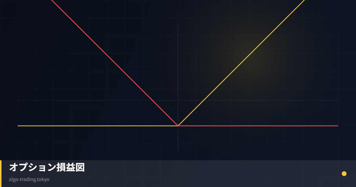
ブラック・ショールズモデルは、ヨーロピアン・オプションの理論価格を算出する基本公式です。ということで、この記事ではPythonで実装し、オプション価格の計算からグリーク指標（デルタ・ガンマ・セータ・ベガ）までをまとめます。

📘 外部参考：Python 公式サイト（ダウンロード） ／ Python 公式ドキュメント（日本語）

📘 外部参考：Getting to Know the “Greeks”（Investopedia）

📘 外部参考：ブラック–ショールズ方程式（Wikipedia 日本語） ／ Black-Scholes Model（Investopedia）

ブラック・ショールズ公式の実装

import numpy as np
from scipy.stats import norm
import pandas as pd

def black_scholes(S, K, T, r, sigma, option_type='call'):
    if T <= 0:
        return max(S - K, 0) if option_type == 'call' else max(K - S, 0)
    d1 = (np.log(S / K) + (r + 0.5 * sigma**2) * T) / (sigma * np.sqrt(T))
    d2 = d1 - sigma * np.sqrt(T)
    if option_type == 'call':
        return S * norm.cdf(d1) - K * np.exp(-r * T) * norm.cdf(d2)
    else:
        return K * np.exp(-r * T) * norm.cdf(-d2) - S * norm.cdf(-d1)

S, K, T, r, sigma = 900, 950, 30/365, 0.05, 0.40
call = black_scholes(S, K, T, r, sigma, 'call')
put_ = black_scholes(S, K, T, r, sigma, 'put')
print(f"コール: {call:.2f}  プット: {put_:.2f}")

グリーク指標の計算

def black_scholes_greeks(S, K, T, r, sigma, option_type='call'):
    if T <= 0:
        return {'delta': 0, 'gamma': 0, 'theta': 0, 'vega': 0}
    d1 = (np.log(S / K) + (r + 0.5 * sigma**2) * T) / (sigma * np.sqrt(T))
    d2 = d1 - sigma * np.sqrt(T)
    gamma = norm.pdf(d1) / (S * sigma * np.sqrt(T))
    vega = S * norm.pdf(d1) * np.sqrt(T) / 100
    if option_type == 'call':
        delta = norm.cdf(d1)
        theta = (-(S * norm.pdf(d1) * sigma) / (2 * np.sqrt(T)) - r * K * np.exp(-r * T) * norm.cdf(d2)) / 365
    else:
        delta = norm.cdf(d1) - 1
        theta = (-(S * norm.pdf(d1) * sigma) / (2 * np.sqrt(T)) + r * K * np.exp(-r * T) * norm.cdf(-d2)) / 365
    return {'delta': round(delta, 4), 'gamma': round(gamma, 6), 'theta': round(theta, 4), 'vega': round(vega, 4)}

greeks = black_scholes_greeks(S, K, T, r, sigma, 'call')
print(greeks)

インプライドボラティリティの逆算

def get_implied_volatility(market_price, S, K, T, r, option_type='call'):
    lo, hi = 0.001, 5.0
    for _ in range(100):
        mid = (lo + hi) / 2
        price = black_scholes(S, K, T, r, mid, option_type)
        if abs(price - market_price) < 0.001:
            return mid
        if price < market_price:
            lo = mid
        else:
            hi = mid
    return mid

market_price = 35.0
iv = get_implied_volatility(market_price, S, K, T, r, 'call')
print(f"インプライドボラティリティ: {iv:.1%}")

シナリオ分析

price_changes = [-0.2, -0.1, 0, 0.1, 0.2]
vol_scenarios = [0.25, 0.40, 0.55]
print("原資産変化 | IV=25% | IV=40% | IV=55%")
print("-" * 45)
for dS in price_changes:
    S_new = S * (1 + dS)
    row_str = f"{dS:+.0%}      "
    for vol in vol_scenarios:
        p = black_scholes(S_new, K, T, r, vol, 'call')
        row_str += f"  {p:7.2f}"
    print(row_str)

まとめ

実際にコードを動かしてみると、ブラック・ショールズの実装自体は思ったより短くなります。インプライドボラティリティの逆算や、原資産変化×IV変化のシナリオテーブルまで作ると実用的だと感じています。